A feature map (\(w \times h \times k\)) can be thought of as a collected 2D array of \(k\)-dimensional patch embeddings, or, equivalently, a coarse image (\(w \times h\)) with \(k\) channels \(f_1, \dots, f_k\). Both CNNs and ViTs, in their respective ways, are in the business of transforming an input image into a sequence of feature maps.

How can we see what a vision encoder sees as an image make its way through its layers? Zero-shot localization methods are designed to generate human-interpretable visualizations from an encoder’s feature maps. These visualizations, which can look like heatmaps or coarse segmentation masks, discriminate between semantically related regions in the input image. The term “zero-shot” refers to the fact that the model has not explicitly been trained on mask annotations for the semantic categories of interest. A vision encoder like CLIP, for instance, has only been trained on image-level text captions.

In this article, we begin with an overview of some early techniques for generating interpretable heatmaps from supervised CNN classifiers, with no additional training required. We then explore the challenges around achieving zero-shot localization with CLIP-style encoders. Finally, we touch on the key ideas behind GEM (Grounding Everything Module) [1], a recently proposed approach to training-free, open-vocabulary localization for the CLIP ViT.

1. Localization with supervised CNN classifiers

Class Activation Maps (2016)

Let’s build some intuition around the concept of localization by considering a simple vision encoder trained for image classification in a supervised way. Assume the CNN uses:

1. Global average pooling (GAP) to transform the final feature map channels \(f_1(x, y), \dots, f_k(x, y)\) into a \(k\)-dimensional vector. In other words, each \(f_i\) is averaged along the width and height dimensions.
2. A single linear layer \(\mathbf{W}\) to map this \(k\)-dimensional vector into a vector of class logits.

The logit for a given class \(c\) can then be written as:

where \(\mathbf{W}_i(c)\) denotes the (scalar) weight of feature channel \(i\) on logit \(c\), and \(Z_i\) is a normalizing constant for the average pooling.

The key observation behind Class Activation Maps [2] is that the above summation can be re-written as:

In other words, the logit can be expressed as a weighted average of the final feature channels, which is then averaged across the width and height dimensions.

It turns out that the weighted average of the \(f_i\)’s alone gives an interpretable heatmap for class \(c\), where larger values match regions in the image that are more semantically related to the class. This coarse heatmap, which can be up-sampled to match the dimensions of the input image, is called a Class Activation Map (CAM):

Intuitively, each \(f_i\) is already a heatmap for some latent concept (or “feature”) in the image - though these do not necessarily discriminate between human-interpretable classes in any obvious way. The weight \(\mathbf{W}_i(c)\) captures the importance of \(f_i\) in predicting class \(c\). The weighted average thus highlights which image features are most relevant to class \(c\). In this way, we can achieve discriminative localization of the class \(c\) without any additional training.

Grad-CAM (2017)

The challenge with class activation maps is that they are only meaningful under certain assumptions about the architecture of the CNN encoder. Grad-CAM [3], proposed in 2019, is an elegant generalization of class activation maps that can be applied to any CNN architecture, as long as the mapping of the final feature map channels \(f_1, \dots, f_k\) to the logit vector is differentiable.

As in the CAM approach, Grad-CAM computes a weighted sum of feature channels \(f_i\) to generate an interpretable heatmap for a class \(c\), but the weight for each \(f_i\) is computed as:

Grad-CAM generalizes the idea of weighing each \(f_i\) proportionally to its importance for predicting the logit for class \(c\), as measured by the average-pooled gradients of the logit with respect to elements \(f_i(x,y)\). Indeed, it can be shown that computing the Grad-CAM weights for a CNN that obeys assumptions 1–2 from the previous section results in the same expression for \(\text{CAM}(c)\) we saw earlier, up to a normalizing constant (see [3] for a proof).

Grad-CAM also goes a step further by applying ReLU on top of the weighted average of the feature channels \(f_i\). The idea is to only visualize features which would strengthen the confidence in the prediction of class \(c\) should their intensity be increased. Once again, the output can then be up-sampled to give a heatmap that matches the dimensions of the original input image.

2. Localization with CLIP

Do these early approaches generalize to CLIP-style encoders? There are two additional complexities to consider with CLIP:

1. CLIP is trained on a large, open vocabulary using contrastive learning, so there is no fixed set of classes.
2. The CLIP image encoder can be a ViT or a CNN.

That said, if we could somehow achieve zero-shot localization with CLIP, then we would unlock the ability to perform zero-shot, open-vocabulary localization: in other words, we could generate heatmaps for arbitrary semantic classes. This is the motivation for developing localization methods for CLIP-style encoders.

Let’s first attempt some seemingly reasonable approaches to this problem given our knowledge of localization using supervised CNNs.

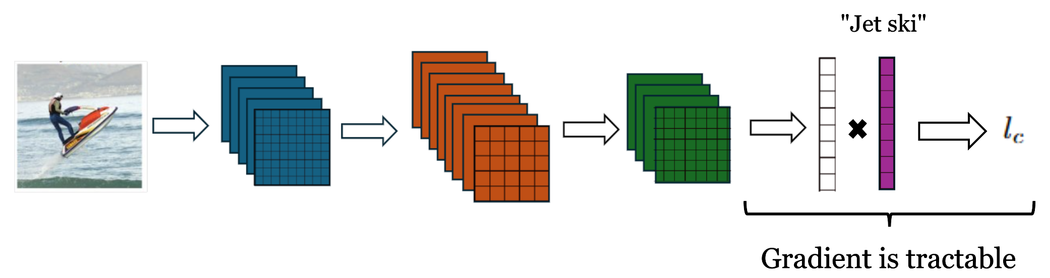
For a given input image, the logit for a class \(c\) can be computed as the cosine similarity between the CLIP text embedding of the class name and the CLIP image embedding. The gradient of this logit with respect to the image encoder’s final feature map is tractable. Hence, one possible approach would be to directly apply Grad-CAM - and this could work regardless of whether the image encoder is a ViT or a CNN.

Another seemingly reasonable approach might be to consider alignment between image patch embeddings and class text embeddings. Recall that CLIP is trained to maximize alignment between an image-level embedding (specifically, the CLS token embedding) and a corresponding text embedding. Is it possible that this objective implicitly aligns a patch in embedding space more closely to text that is more relevant to it? If this were the case, we could expect to generate a discriminative heatmap for a given class by simply visualizing the similarity between its text embedding and each patch embedding:

Opposite Visualizations

Interestingly, not only do both these approaches fail, but the resulting heatmaps turn out to be the opposite of what we would expect. This phenomenon, first described in the paper “Exploring Visual Explanations for Contrastive Language-Image Pre-training” [4], has been observed consistently across different CLIP architectures and across different classes. To see examples of these “opposite visualization” with both patch-text similarity maps and Grad-CAM, take a look at page 19 in the pre-print “A Closer Look at the Explainability of Contrastive Language-Image Pre-training” [5]. As of today, there is no single, complete explanation for this phenomenon, though some partial hypotheses have been proposed.

Self-Attention Maps

One such hypothesis is detailed in the aforementioned paper [5]. This work restricts its scope to the ViT architecture and examines attention maps in the final self-attention block of the CLIP ViT. For a given input image and text class, these attention maps (\(w \times h\)) are computed as follows:

1. The patch embedding (a \(d\)-dimensional vector - the same as the output dimension of the image-level embedding) with highest cosine similarity to the class text embedding is selected as an anchor patch.
2. The attention map is obtained by computing the query-key attention weights for the anchor patch query embedding \(Q\) and all key embeddings \(K\), which can be reshaped into a heatmap of size \(w \times h\). The attention weights are computed as:

You might expect the anchor patch to be attending mostly to other patches in the image that are semantically related to the class of interest. Instead, these query-key attention maps reveal that anchor patches consistently attend to unrelated patches just as much. As a result, query-key attention maps are blotchy and difficult to interpret (see the paper [5] for some examples). This, the authors suggest, could explain the noisy patch-text similarity maps observed in the CLIP ViT.

On the other hand, the authors find that value-value attention maps are more promising. Empirically, they show that value-value attention weights are larger exclusively for patches near the anchor that are semantically related to it. Value-value attention maps are not complete discriminative heatmaps, but they are a more promising starting point.

3. Grounding Everything Module (2024)

Hopefully, you can now see why training-free localization is not as straightforward for CLIP as it was for supervised CNNs - and it is not well-understood why. That said, a recent localization method for the CLIP ViT called the Grounding Everything Module (GEM) [1], proposed in 2024, achieves remarkable success. GEM is essentially a training-free method to correct the noisy query-key attention maps we saw in the previous section. In doing so, the GEM-modified CLIP encoder can be used for zero-shot, open-vocabulary localization. Let’s explore how it works.

Self-Self Attention

The main idea behind GEM is called self-self attention, which is a generalization of the concept of value-value attention.

Given queries \(Q\), keys \(K\) and values \(V\), the output of a self-self attention block is computed by applying query-query, key-key, and value-value attention iteratively for \(t = 0, \dots, n\):

where \(p_0 \in \{Q, K, V\}\) and \(n\), the number of iterations, is a hyperparameter. This iterative process can be thought of as clustering the initial tokens \(p_0\) based on dot-product similarity. By the end of this process, the resulting tokens \(p_n\) is a set of cluster “centers” for the initial tokens \(p_0\).

The resulting self-self attention weights are then ensembled to produce the output of the self-self attention block:

where:

This is in contrast to a traditional query-key attention block, whose output is computed simply as:

Grounding Everything Module

Now consider our method for generating value-value attention maps in the previous section, where we first chose an anchor patch based on similarity to a class text embedding, then computed value-value attention map. GEM can be thought of as the reverse of this process, where:

1. The first step is to apply qkv-ensembled self self-attention instead of regular attention for the last \(m\) attention blocks in the ViT (\(m\) is another hyperparameter). Intuitively, this is a way to compute ensembled cluster assignments for value embeddings \(V\), thereby correcting the original query-key attention maps.
2. The second step is to generate a heatmap by computing the cosine similarity between patch embeddings output from the modified ViT and the class text embedding. This effectively gives a class logit for each cluster.

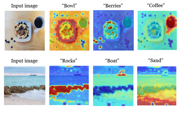
This set of logits can then be reshaped to produce a discriminative heatmap for the chosen class, which can take the form of any arbitrary text! Below are some examples of GEM heatmaps for various class prompts (red indicates higher similarity to the class prompt):

Discriminative localization can transform an image-level encoder into a model that can be used for semantic segmentation, without the need for notoriously expensive mask annotations. Moreover, training-free localization is a powerful approach to making vision encoders more explainable, allowing us to see what they see.

For supervised vision models, zero-shot localization began with class activation maps, a technique for a specific kind of CNN architecture. Later, a generalization of this approach, applicable to any supervised CNN architecture, was proposed. When it comes to CLIP-style encoders, however, training-free localization is less straightforward: the phenomenon of opposite visualizations remains largely unexplained and exists across different CLIP encoder architectures. As of today, some localization techniques for the CLIP ViT such as GEM have proven successful. Is there a more generalized approach waiting to be discovered?

References

• W. Bousselham, F. Petersen, V. Ferrari, H. Kuehne, Grounding Everything: Emerging Localization Properties in Vision-Language Transformers (2024), 2024 IEEE Conference on Computer Vision and Pattern Recognition (CVPR)
• B. Zhou, A. Khosla, A. Lapedriza, A. Oliva, A. Torralba, Learning Deep Features for Discriminative Localization (2016), 2016 IEEE Conference on Computer Vision and Pattern Recognition (CVPR)
• R. R. Selvaraju, M. Cogswell, A. Das, R. Vedantam, D. Parikh, D. Batra, Grad-CAM: Visual Explanations from Deep Networks via Gradient-based Localization (2017), 2017 IEEE International Conference on Computer Vision (ICCV)
• Y. Li, H. Wang, Y. Duan, H. Xu, X. Li, Exploring Visual Explanations for Contrastive Language-Image Pre-training (2022)
• Y. Li, H. Wang, Y. Duan, J. Zhang, X. Li, A Closer Look at the Explainability of Contrastive Language-Image Pre-training (2024)

In this article, we will explore the inductive biases that go into designing effective position encoders for geographic coordinates. Position on Earth can be a useful input to a wide range of prediction tasks, including image classification. As we will see, using latitude and longitude directly as input features is under-constraining and ultimately will make it harder for the model to learn anything meaningful. Instead, it is more common to encode prior knowledge about latitude and longitude in a nonparametric re-mapping that we call a positional encoder.

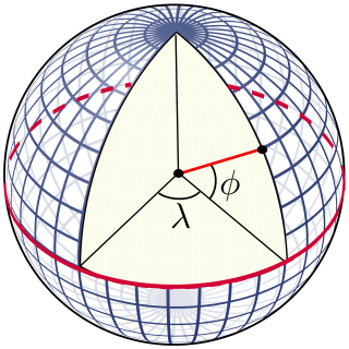
We want to train a neural network to predict some variable of interest given a position on the surface of the Earth. How should we encode a position \((\lambda, \phi)\) in spherical coordinates – i.e. a longitude/latitude pair – into a vector that can be used as an input to our network?

By Peter Mercator, Public Domain.

Simple approach

One possible approach would be to use latitude and longitude values directly as inputs. In this case our input feature space would be the rectangle \([-\pi, \pi] \times [0, \pi]\), which I will refer to as lat/lon space. As with position encoders for transformers, this simple approach unfortunately has its limitations:

1. Notice that as you move towards the poles, the distance on the surface of the Earth covered by 1 unit of longitude (\(\lambda\)) decreases. Lat/lon space does not preserve distances on the surface of the Earth.
2. Notice that the position on Earth corresponding to coordinates \((\lambda, \phi)\) should be identical to the position corresponding to \((\lambda + 2\pi, \phi)\). But in lat/lon space, these two coordinates are very far apart. Lat/lon space does not preserve periodicity: the way spherical coordinates wrap around the surface of the Earth.

To learn anything meaningful directly from inputs in lat/long space, a neural network must learn how to encode these properties about the curvature of the Earth’s surface on its own – a challenging task. How can we instead design a position encoder that already encodes these inductive biases? Let’s explore some early approaches to this problem and how they have evolved over time.

Early Position Encoders

Discretization-based (2015)

The first paper to propose featurizing geographic coordinates for use as input to a convolutional neural network is called “Improving Image Classification with Location Context” [3]. Published in 2015, this work proposes and evaluates many different featurization approaches with the goal of training better classification models for geo-tagged images.

The idea behind each of their approaches is to directly encode a position on Earth into a set of numerical features that can be computed from auxiliary data sources. Some examples include:

• Dividing the U.S. into evenly spaced grids in lat/lon space and using a one-hot encoding to encode a given location into a vector based on which grid it falls into.
• Looking up the U.S ZIP code that corresponds to a given location, then retrieving demographic data about this ZIP code from ACS (American Community Survey) related to age, sex, race, living conditions, and more. This is made into a numerical vector using one-hot encodings.
• For a chosen set of Instagram hashtags, counting how many hashtags are recorded at different distances from a given location and concatenating these counts into a vector.
• Retrieving color-coded maps from Google Maps for various features such as precipitation, land cover, congressional district, and concatenating the numerical color values from each into a vector.

Note that these positional encodings are not continuous and do not preserve distances on the surface of the Earth. In the first example, two nearby locations that fall into different grids will be equally distant in feature space as two locations from opposite sides of the country. Moreover, these features mostly rely on the availability of auxiliary data sources and must be carefully hand-crafted, requiring a specific choice of hashtags, map features, survey data, etc. These approaches do not generalize well to arbitrary locations on Earth.

WRAP (2019)

In 2019, a paper titled “Presence-Only Geographical Priors for Fine-Grained Image Classification” [4] took an important step towards the geographic position encoders commonly used today. Similar to the work from the previous section, this paper studies how to use geographic coordinates for improving image classification models.

The key idea behind their position encoder is to leverage the periodicity of sine and cosine functions to encode the way geographic coordinates wrap around the surface of the Earth. Given latitude and longitude \((\lambda, \phi)\), both normalized to the range [-1, 1], the WRAP position encoder is defined as:

Unlike the approaches in the previous section, WRAP is continuous and easily computed for any position on Earth. The paper then shows empirically that training a fully-connected network on top of these features and combining them with latent image features can lead to improved performance on fine-grained image classification benchmarks.

The Double Fourier Sphere Method

The WRAP encoder appears simple, but it successfully encodes a key inductive bias about geographic position while remaining expressive and flexible. In order to see why this choice of position encoder is so powerful, we need to understand the Double Fourier Sphere (DFS) method [5].

DFS is a method of transforming any real-valued function \(f(x, y, z)\) defined on the surface of a unit sphere into a \(2\pi\)-periodic function defined on a rectangle \([-\pi, \pi] \times [-\pi, \pi]\). At a high level, DFS consists of two steps:

1. Re-parametrize the function \(f(x, y, z)\) using spherical coordinates, where \((\lambda, \phi) \in [-\pi, \pi] \times [0, \pi]\)

   \[f(\lambda, \phi) = f(\cos\lambda \sin\phi, \sin\lambda \sin\phi, \cos\phi)\]

2. Define a new piece-wise function over the rectangle \([-\pi, \pi] \times [-\pi, \pi]\) based on the re-parametrized \(f\) (essentially “doubling it over”).

Notice that the DFS re-parametrization of the Earth’s surface (step 1.) preserves the properties we discussed earlier. For one, as \(\phi\) tends to 0 or \(\pm\pi\) (the Earth’s poles), the distance between two points \((\lambda, \phi)\) and \((\lambda', \phi)\) after re-parametrization decreases. Moreover, the re-parametrization is periodic and smooth.

Fourier Theorem

It is a fact that any continuous, periodic, real-valued function can be represented as a weighted sum of sines and cosines. This is called the Fourier Theorem, and this weighted sum representation is called a Fourier series. It turns out that any DFS-transformed function can be represented with a finite set of sines and cosines. They are known as DFS basis functions, listed below:

Here, \(\cup\) denotes union of sets, and \(S\) is a collection of scales (i.e. frequencies) for the sinusoids.

DFS-Based Position Encoders

Notice that the set of DFS basis functions includes the four terms in the WRAP position encoder. “Sphere2Vec” [4] is the earliest publication to observe this, proposing a unified view of position encoders based on DFS. In fact, with this generalization in mind, we can construct a geographic position encoder by choosing any subset of the DFS basis functions – WRAP is just one such choice. Take a look at [5] for a comprehensive overview of various DFS-based position encoders.

Why are DFS-based encoders so powerful?

Consider what happens when a linear layer is trained on top of a DFS-based position encoder: each output element of the network is a weighted sum of the chosen DFS basis functions. Hence, the network can be interpreted as a learned Fourier series. Since virtually any function defined on the surface of a sphere can be transformed using the DFS method, it follows that a linear layer trained on top of DFS basis functions is powerful enough to encode arbitrary functions on the sphere! This is akin to the universal approximation theorem for multilayer perceptrons.

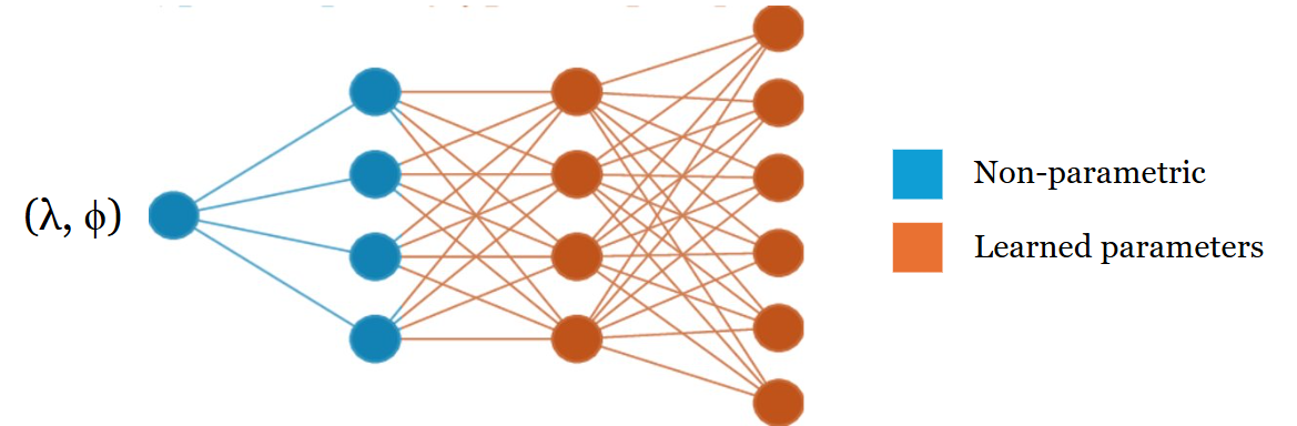
In practice, only a small subset of the DFS basis functions is used for the position encoder and a fully-connected network is trained on top of these. The composition of a non-parametric position encoder with a neural network is commonly referred to as a location encoder:

Geographic Location Encoders Today

As we have seen, a DFS-based position encoder can effectively encode inductive biases we have about the curvature of the Earth’s surface. One limitation of DFS-based encoders is that they assume a rectangular domain \([-\pi, \pi] \times [-\pi, \pi]\). While this is mostly fine since the DFS re-parametrization already accounts for how distances get warped closer to the poles, this assumption breaks down at the poles themselves (\(\phi = 0, \pm\pi\)), which are lines in the rectangular domain that collapse to singular points on the Earth’s surface.

A different set of basis functions called spherical harmonics have recently emerged as an alternative. Spherical harmonics are basis functions that are natively defined on the surface of the sphere as opposed to a rectangle. They have been shown to exhibit fewer artifacts around the Earth’s poles compared to DFS-based encoders [5]. Notably, spherical harmonics are the basis functions used in the SatCLIP location encoder [6], a recent foundation model for geographic coordinates trained in the style of CLIP.

Though geographic position encoders began with discrete, hand-crafted features in the 2010s, these do not easily generalize to arbitrary locations and require domain-specific metadata such as land cover and demographic data. Today, geographic coordinates are much more commonly used as neural network inputs because simple yet meaningful and expressive ways of encoding them have emerged. With the rise of web-scale datasets which are often geo-tagged, the potential for using geographic coordinates as inputs for prediction tasks is now immense.

References

[1] K. Tang, M. Paluri, L. Fei-Fei, R. Fergus, L. Bourdev, Improving Image Classification with Location Context (2015)

[2] O. Mac Aodha, E. Cole, P. Perona, Presence-Only Geographical Priors for Fine-Grained Image Classification (2019)

[3] Double Fourier Sphere Method, Wikipedia

[4] G. Mai, Y. Xuan, W. Zuo, K. Janowicz, N. Lao, Sphere2Vec: Multi-Scale Representation Learning over a Spherical Surface for Geospatial Predictions (2022)

[5] M. Rußwurm, K. Klemmer, E. Rolf, R. Zbinden, D. Tuia, Geographic Location Encoding with Spherical Harmonics and Sinusoidal Representation Network (2024), ICLR 2024

[6] K. Klemmer, E. Rolf, C. Robinson, L. Mackey, M. Rußwurm, SatCLIP: Global, General-Purpose Location Embeddings with Satellite Imagery (2024)

Here, \(X_i = [ x_{i1} x_{i2} \dots x_{id} ]\) are the features (also called covariates) of an input we want to classify. For example, these could be the pixels of an image, or a vector representation of some text. We’ll also assume \(x_{i1} = 1\), so as to include a bias term in our model. \(\beta\) is a \(d\)-dimensional column vector of our learnable model parameters, and \(\hat y_i\) is the model output. The function \(\sigma\) is the sigmoid function, and it is given by:

In an introductory ML course, the sigmoid function is produced seemingly out of nowhere, and it happens to be exactly what we need to make our model work:

• The range of \(\sigma\) is \((0, 1)\), which means our model output \(\hat y_i\) can be interpreted as a probability distribution (more on this later). Hence our model can make classification predictions simply by rounding \(\hat y_i\) to the nearest integer, either 0 or 1.
• \(\sigma\) is differentiable everywhere, and its derivative can be elegantly expressed as \(\sigma'(z) = \sigma(z)(1 - \sigma(z))\). In particular the derivative is nowhere 0, because \(\sigma(z)\) is within \((0,1)\) for any \(z\). This is a useful property if we are training our model using gradient descent.

But certainly sigmoid isn’t the only differentiable function to possess these desirable properties. What makes sigmoid so well-suited for binary classification? Where does the expression for sigmoid \(\eqref{eq1}\) come from? In the following sections I will present an answer to these questions from a statistical perspective, and explain why sigmoid is in fact the most “natural” choice for our binary classification model.

The Exponential Family

We begin with an overview of the exponential family of distributions, perhaps a seemingly unrelated topic. A probability distribution with density \(p(x \vert \theta)\) is said to belong to the exponential family if \(p(x \vert \theta)\) can be written in the following form:

• \(\theta\) could be any set of parameters, and \(\eta\) is a reparametrization function. The parameters \(\eta(\theta)\) are called the natural parameters (or canonical parameters) of the distribution.
• \(T(x)\) is called the sufficient statistic for the distribution (we’ll see why).
• \(A(\eta(\theta))\) is called the cumulant function. It can be interpreted as a normalization constant for the PDF.
• \(h(x)\) could be any nonnegative function.

It turns out that many common distributions belong to the exponential family, including the Bernoulli, Gaussian, Poisson, Gamma, and Beta distributions.

Example: Bernoulli Distribution

As an example, let’s see how the PDF of the Bernoulli distribution can be expressed in the form of \(\eqref{eq2}\). A common expression for the PDF of the Bernoulli is:

where \(\theta\) is a parameter in \([0, 1]\). This gives:

Note that \(\eqref{eq3}\) is in the desired form \(\eqref{eq2}\):

• \(\eta(\theta) = \log\big(\frac{\theta}{1-\theta}\big)\) is the natural parameter
• \(T(x) = x\) is the sufficient statistic
• \(A(\eta(\theta)) = - \log (1 - \theta)\) is a normalizing constant
• $h(x) = 1$

In this example, \(\theta\) is called the mean parameter of the Bernoulli distribution. In general, distributions in the exponential family have mean parameters which are not necessarily equal to their natural parameters. Formally, the mean parameters of a distribution in the exponential family are defined as \(\theta := \mathbb{E}_{x \sim p}[T(x)]\) , the expected value of the sufficient statistic. Note that since \(T(x) = x\) for the Bernoulli distribution, this definition coincides with our intuition for the mean parameter of a Bernoulli distribution being the expected success rate: \(\theta = \mathbb{E}_{x \sim p}[x]\). As another example, the mean parameters of the Gaussian distribution are the familiar \(\theta = [ \mu \sigma^2 ]\), while its natural parameters are the (perhaps not-so-natural) \([\frac{\mu }{\sigma ^{2}}{\frac {1}{2\sigma ^{2}}}]\).

Sufficient Statistics

Why should we care about the exponential family? One reason is that their sufficient statistics are easy to determine, which makes them valuable for parametric inference. Recall that a statistic is any function of random samples \(X\) from a distribution. Informally, a statistic \(T(X)\) is sufficient for a distribution \(p(x \vert \theta)\) if we can estimate parameters \(\theta\) using \(T(X)\), and if there is no further information we can obtain from \(X\) about \(\theta\) that is not already included in \(T(X)\).

As an example, consider the Bernoulli distribution once again, parametrized by \(\theta\). If we sample \(x_1,...x_n \stackrel{iid}{\sim} Bernoulli(\theta)\), then knowing the sample mean \(\frac{1}{n} \sum_{i=1}^n x_i\) is enough to estimate \(\theta\). Indeed, the MLE estimate for \(\theta\) is \(\hat \theta = \frac{1}{n} \sum_{i=1}^n x_i\). Knowing anything more about \(x_1,...,x_n\) could not give us a better estimate for \(\theta\). We say that \(\sum_{i=1}^n x_i\) is a sufficient statistic for the Bernoulli distribution (assuming \(n\) is known beforehand).

Notice that the joint distribution of samples \(x_1,...,x_n\) drawn \(iid\) from an arbitrary distribution in the exponential family is:

In the previous section we showed \(T(x) = x\) for the Bernoulli distribution. It follows that \(\sum_{i=1}^n T(x_i) = \sum_{i=1}^n x_i\) is precisely the sufficient statistic for the Bernoulli distribution! It can be shown that in the general case as well, \(\sum_{i=1}^n T(x_i)\) is a sufficient statistic for any distribution in the exponential family.

Hence, all the information needed to estimate the parameters of an exponential-family distribution from \(iid\) samples \(x_1,...,x_n\) is contained in a single vector \(\sum_{i=1}^n T(x_i)\) of fixed dimension (as opposed to dimension that grows with sample size \(n\)), and this vector can simply be read off the PDF \(\eqref{eq4}\) of the joint distribution. As an aside, it turns out that much more is true. The Pitman-Koopman-Darmois theorem states that the exponential family of distributions is the only family of distributions (under a few mild assumptions) for which the sufficient statistics are finite-dimensional for arbitrarily large sample sizes.

Reparametrizing

Earlier, we computed a reparametrization \(\eta(\theta) = \log\big(\frac{\theta}{1-\theta}\big)\) of the Bernoulli PDF which mapped its mean parameter \(\theta\) to its natural parameter. Notice furthermore that the mapping is invertible, with inverse given by (does this look familiar?):

It is now natural to ask whether it is always possible to reparametrize from the natural parameters \(\eta\) to the mean parameters \(\theta = \mathbb{E}_{x \sim p}[T(x)]\) for any distribution in the exponential family. If \(\theta\) are the mean parameters, can we always find an \(\eta(\theta)\) that is one-to-one? As it turns out, we can. Yet another beautiful property satisfied by any distribution in the exponential family is the following:

Here, \(\eta := \eta(\theta)\) denotes the natural parameters and \(A(\eta)\) is the cumulant function. Note that \(\eqref{eq5}\) is precisely the expression for the mean parameters \(\theta\), so we can write \(\eqref{eq6}\) as:

Since the variance \(\text{Var}_{x \sim p}[T(x)]\) is a strictly positive quantity, it follows that \(\dfrac{\partial \theta(\eta)}{\partial \eta} > 0\).

Therefore, we can always express the mean parameters \(\theta\) as a function of \(\eta\) (the function given by \(\eqref{eq5}\)), and this function is guaranteed to be strictly increasing, hence invertible.

The Generalized Linear Model

Classification, Revisited

In the introduction, we considered the logistic regression model from a discriminative perspective: our model was a function of input features, parametrized by \(\beta\), that would make predictions to distinguish (“discriminate”) between inputs from different classes. Suppose we now consider the same model, from a generative perspective. We assume that conditioned on the input features \(X_i\), the true class \(y_i\) of an input was drawn by some generative process from a Bernoulli distribution with unknown mean parameter \(\theta_i\). We have observed \(X_1,...,X_n\) and \(y_1,...,y_n\). Our goal is to learn \(\beta\) so we can predict a likely estimate for each \(\theta_i\). Here is this model:

Generalized Linear Model

As we now know quite well, the Bernoulli distribution belongs to the more general exponential family. We have seen how numerous properties of the Bernoulli distribution could be generalized to arbitrary distributions in the exponential family, including the formula for a sufficient statistic, and the invertibility of \(\eta(\theta)\) when \(\theta\) are the mean parameters. Can we generalize our classification model as well?

In \(\eqref{eq7}\) we are modeling the mean parameter of the Bernoulli distribution. Instead, let’s choose an arbitrary distribution \(p(x \vert \theta)\) in the exponential family, parametrized by its mean parameters \(\theta\), and model these. For simplicity we assume the mean parameter \(\theta\) is one-dimensional, as in the Bernoulli distribution. We also replace \(\sigma\) in \(\eqref{eq7}\) with an arbitrary invertible function \(g^{-1}\). Here is the resulting model:

We have just constructed the Generalized Linear Model! The Generalized Linear Model (GLM) is a model for the mean parameters of an arbitrary distribution in the exponential family. The model is specified by three components:

• The distribution \(p(\cdot \vert \theta)\): a distribution from the exponential family parametrized by its mean parameters \(\theta\)
• The link function \(g(\theta)\): an invertible function of the mean parameters \(\theta\)
• Covariates \(X\) and a linear predictor \(X\beta\), where \(\beta\) are the model parameters

Notice that our model “works” precisely because of the elegant properties of the exponential family described earlier. We always know what a sufficient statistic looks like for a distribution in the exponential family, and in particular we know that it will always be of a fixed dimension. Therefore it is feasible to model the mean parameters \(\theta\), which correspond to the expectation of the sufficient statistic. We also know that there is an invertible parametrization \(\theta(\eta)\) of the mean parameters, so we will be able to recover an estimate for the natural parameters \(\eta\) if we can estimate \(\theta\).

The power of the GLM is in its generality. While the logistic regression model could only model binary data, the GLM provides a framework to model response data drawn from any distribution in the exponential family (and by the Pitman-Koopman-Darmois theorem, drawn from any distribution with sufficient statistics of fixed dimension). We can now model count data with the Poisson distribution, wait times with Gamma, multi-class data with the Multinomial. In addition, the GLM is consistent with other well-known models: with the Gaussian distribution, for instance, we can recover traditional linear regression.

On the flipside, the generality of the GLM may also seem daunting. We now have so much more freedom in specifying our model. For example, how do we choose a link function \(g\)? In general there are several possible options for the link function for a given distribution, and each has their own advantages. In the next section we will examine a special choice for the link function.

The Canonical Link

The canonical link is the link function that results in the natural parameters \(\eta\) themselves being modeled as a linear function \(X\beta\) of the covariates. To be precise, the canonical link function is simply \(g(\theta) = \eta(\theta)\).

This is a cute definition, but it might seem like another trick pulled out of a hat. What makes this choice of link function so special? We will prove the following result:

Proposition: Suppose we have a GLM where the canonical link function \(g\) is used, and the specified distribution satisfies \(T(y) = y\). Then the MLE estimate \(\hat \beta\) satisfies the orthogonality condition \(\sum_{i=1}^n (y_i - \hat \theta_i)X_i = 0\), where \(\hat \theta_i = g^{-1}(X_i \hat \beta)\).

Proof. Given \(iid\) samples \((X_1, y_1), ..., (X_n, y_n)\) where the \(y_i\)’s are distributed according to the specified exponential-family distribution, the log-likelihood for this data is:

The canonical link function is \(g(\theta) = \eta(\theta)\), and under our model we have \(g(\hat \theta_i) = X_i \hat \beta\). Plugging this in gives:

Now we differentiate \(\eqref{eq8}\) with respect to \(\beta\) and set the derivative to 0 (using \(\eqref{eq5}\)), since this condition must be satisfied by the MLE \(\hat \beta\):

This is the orthogonality condition, as required. \(\blacksquare\)

Note that with the assumption \(T(y) = y\), the mean parameter \(\theta_i\) is precisely the expected value of \(y_i\). Let \(\epsilon_i := y_i - \hat \theta_i\). This corresponds to the leftover noise in our observations \(y_i\) that has not been explained by our model of their means \(\theta_i\). Now recall that the feature vectors \(X_i = [x_{i1} x_{i2} \dots x_{id}]\) have \(x_{i1} = 1\), so as to include a bias term in our linear predictor. Examining the vector equality \(\eqref{eq9}\) along the first component, it follows that \(\bar \epsilon := \sum_{i=1}^n \epsilon_i = 0\). Hence, with \(\bar x_{\cdot j} := \sum_{i=1}^n x_{ij}\), for each covariate \(x_{\cdot j}\) we have:

(Here \(\text{Cov}(\cdot)\) denotes the sample covariance.)

The unexplained noise \(\epsilon_i\) and each covariate \(x_{ij}\) are uncorrelated! In other words, all the linear dependence of \(\theta_i\) on \(X_i\) has been “explained away” by our model under the assumptions we made. This is intuitively a very natural and desirable property for our optimal model parameters to satisfy. As a final note, the assumption \(T(y) = y\) that we needed for this proof holds for many common distributions, including Bernoulli (as we have seen), Normal, Poisson, and Gamma distributions.

Why Sigmoid?

We now return to the world of machine learning and the question that motivated our study of GLMs: why sigmoid? As you may have noticed, the sigmoid function is the inverse of the canonical link function for the Bernoulli distribution. Earlier in this section we saw that we can cast the binary classification task as a parametric inference problem for a GLM. In the latter setting, we estimate our parameters \(\beta\) by maximizing the joint likelihood of our observations. In a machine learning setting, when training a binary logistic classifier, we typically minimize the cross-entropy loss (dependence on \(\beta\) is implicit in the formula):

It is easy to see that \(\mathcal{L}_{CE}\) is exactly the average negative log-likelihood of observations \((X_i, y_i)\) under a Bernoulli distribution parametrized by \(\hat \theta_i = \sigma(X_i\beta)\). Hence, gradient descent on this objective is equivalent to iteratively maximizing the log-likelihood of a Bernoulli GLM with canonical link function! Using the canonical link, namely the sigmoid function, ensures the optimal parameters \(\hat \beta\) will satisfy the desirable orthogonality condition. Moreover, the expression of the gradient of \(\mathcal{L}_{CE}\) is as given in \(\eqref{eq9}\). As an added bonus, we can thus interpret gradient descent on \(\mathcal{L}_{CE}\) as an iteratively re-weighted least squares algorithm. This is in fact identical to the procedure that statisticians use to fit GLMs; see Nelder and Wedderburn (1972) for more on this.

Recap

From a machine learning perspective, we can intuitively convince ourselves that sigmoid and cross-entropy loss possess some desirable properties for classification and learning using gradient descent. As it happens, all our intuition can be formalized through the theory of Generalized Linear Models, and we find that sigmoid and cross-entropy loss are truly the most natural choices. Here is a summary of what we have seen:

1. A distribution (under some additional conditions) belongs to the exponential family if and only if there is a vector of sufficient statistics that has fixed dimension when sample size increases. We can always reparametrize a distribution in the exponential family with the mean parameters instead of the natural parameters. The mean parameters are defined as the expected value of the sufficient statistic, and are therefore finite-dimensional.
2. Due to these nice properties of the exponential family, we can construct the Generalized Linear Model, which models the mean parameters of a distribution from the exponential family as a linear function of input features passed through a possibly nonlinear link function. In general there can be several possible choices for the link function for a given distribution.
3. The canonical link is the link function which results in the natural parameters themselves being modeled as a linear function of the input features. When using the canonical link function, the MLE estimate for the model parameters satisfies some convenient and desirable properties.
4. The logistic regression model is a special case of a GLM with Bernoulli distribution. Using the canonical link for this model is equivalent to using sigmoid activation, and cross-entropy loss is exactly equal to the negative log-likelihood for the GLM. Hence our standard binary classification model enjoys all the aforementioned desirable properties of the GLM with canonical link.

References

• J. A. Nelder and R. W. M. Wedderburn (1972), Generalized Linear Models, Journal of the Royal Statistical Society. (pdf)
• Kevin P. Murphy (2013) Machine Learning: A Probabilistic Perspective. (Ch. 9)
• Probabilistic Graphical Model lecture slides, CMU (pdf)
• David Blei, “Exponential Families” (pdf)
• CSC412 Winter 2020 Course Notes, University of Toronto (link)
• Probabilistic ML lecture notes, Princeton University (pdf)
• Generalized Linear Models lecture slides, University of Michigan (pdf)